Consideration of LCR PHONO EQUALIZER

How to determine the constants of a constant impedance LCR type phono equalizer (RIAA curve and other equalizing curves)

This article was originally written in Japanese in 2022 and has been retranslated into English in 2025.

1. Introduction

I’m not planning on making one right now, but while browsing audio-related websites, I came across the LCR phono equalizer coils from Hashimoto Transformers and Noguchi Transformers, and while looking at the recommended circuit diagram (Hashimoto Electric H-EQL), I wanted to analyze what kind of playback curve would be obtained with those constants.

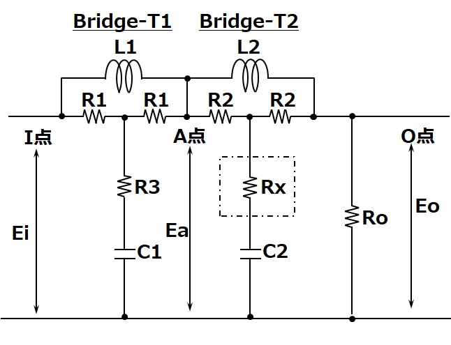
The circuit shown here is the original circuit that makes up the LCR equalizer. The LCR equalizer coil requires optimal L (inductance) values ​​for low frequencies (turnover) and high frequencies (roll-off) to obtain RIAA playback characteristics under conditions of input/output impedance of 600Ω.

This original circuit is a constant impedance circuit with input/output impedance of 600Ω for the first and second stages. If you look at each circuit, you will see that it is a bridge T-type circuit configuration. This is basically the same as a bridge T-type attenuator, with the two sets of variable resistors replaced with L and C. Under the condition that the total impedance is constant, the attenuator changes the amount of attenuation by changing the combination of resistance values. It is best to think of this as replacing the combination of resistance values ​​with the change in the frequency response characteristics for the selected L and C.

Both Bridge-T1 and Bridge-T2 in the diagram are constant impedance bridge T circuits. In other words, the impedance when looking at the load (output) side from the input point I, the intermediate point A, and the output point O is constant and matches the output resistance Ro. Therefore, the LCR constants of Bridge-T1 and 2 can be calculated independently, and the order can be changed.

Since there is L between the input and output and C on the common terminal side, it is easy to understand intuitively that the output of this Bridge-T1 and 2 circuit decreases as the frequency increases.

2. Analysis of Bridge-T1 circuit

To simplify the calculation, the above Bridge-T circuit is converted to the following Y-type circuit.

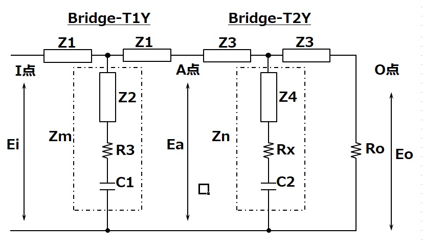
The Δ-Y conversion is simply calculated according to the conversion formula.

Z1＝jωL1R1/(jωL1+2R1) 　　 Equation (2.1)
Z2=R1^2/(jωL1+2R1) 　　　　 Equation (2.2)
Zm=Z2+R3+1/(jωC1) 　　　　　 Equation (2.3)

The impedance seen from point A to the load side is the same as the final load, so it is Ro regardless of the next stage (Bridge-T2). The impedance seen from point I on the input side is also Ro, so

Ztotal＝Ro＝Z1+Zm//(Z1+Ro)＝Z1+Zm(Z1+Ro)/(Z1+Zm+Ro) 　　　　　Equation (2.4)
(Ro-Z1)(Z1+Zm+Ro)=Zm(Z1+Ro)
Ro^2-Z1^2+Zm(Ro-Z1)=Zm(Z1+Ro)
Ro^2=Z1^2+Zm(Z1+Ro-Ro+Z1) Ro^2=Z1(Z1+2Zm) 　　　　　 Equation (2.6)
Zm=(Ro^2-Z1^2)/(2Z1) 　　　　　 Equation (2.7)
2Z1Zm＝Ro^2-Z1^2
Ro^2＝2Z1Zm+Z1^2

Here, we rationalize the denominators of Z1 and Z2, and then calculate Zm.

Z1＝(jωL1R1)/(2R1+jωL1)
=(jωL1R1)(2R1-jωL1)/( (2R1)^2-(jωL1)^2 )
=(ω^2L1^2R1+j2ωL1R1^2)/( (ωL1)^2+(2R1)^2 )
=(ω^2L1^2R1+j2ωL1R1^2)/(ω^2L1^2+4R1^2)
=ωL1R1(ωL1+2jR1)/(ω^2L1^2+4R1^2)
Z1=R1ωL1(ωL1+2jR1)/(ω^2L1^2+4R1^2) Equation (2.8)
Z2＝R1^2/(2R1+jωL1) =R1^2(2R1-jωL1)/((2R1+jωL1)(2R1-jωL1))
=R1^2(2R1-jωL1)/(ω^2L1^2+4R1^2) Equation (2.9)
Zm＝Z2+R3+1/(jωC1)
=R1^2(2R1-jωL1)/(ω^2L1^2+4R1^2)+R3+1/(jωC1)
= (R1^2(2R1-jωL1)+R3(ω^2L1^2+4R1^2)+(ω^2L1^2+4R1^2)/(jωC1))/ (ω^2L1^2+4R1^2) =(2R1^2(R1+2R3)+ω^2L1^2R3-j(ωL1R1^2+(ω^2L1^2+4R1^2)/(ωC1)))/(ω^2L1^2+4R1^2) Equation (2.10)
From Ro^2=Z1(Z1+2Zm) (2.6 derived)
Z1+2Zm=(ωL1R1(ωL1+2jR1)+2(2R1^2(R1+2R3)+ω^2L1^2R3-j(ωL1R1^2+(ω^2L1^2+4R1^2)/(ωC1))))/(ω^2L1^2+4R1^2)
=(ω^2L1^2R1+2jωL1R1^2+4R1^2(R1+2R3)+2ω^2L1^2R3- 2j(ωL1R1^2+(ω^2L1^2+4R1^2)/(ωC1))))/(ω^2L1^2+4R1^2) =(ω^2L1^2R1+2ω^2L1^2R3+4R1^2(R1+2R3)-2j(ωL1R1^2+(ω^2L1^2+4R1^2)/(ωC1)))+2jωL1R1^2)/(ω^2L1^2+4R1^2)
=( ω^2＊L1^2(R1+2R3)+4R1^2(R1+2R3)-2j(ωL1R1^2-ωL1R1^2+(ω^2L1^2+4R1^2)/(ωC1)) ) /(ω^2L1^2+4R1^2)
=( (R1+2R3)(ω^2L1^2+4R1^2)-2j(ω^2L1^2+4R1^2)/(ωC1) ) /(ω^2L1^2+4R1^2) =(R1+2R3)-2j/(ωC1)
Ro^2=Z1(Z1+2Zm)=R1ωL1(ωL1+2jR1)/(ω^2L1^2+4R1^2) * ((R1+2R3)-2j/(ωC1) )
=((ω^2L1^2R1+j2ωL1R1^2)(R1+2R3)-2j(ω^2L1^2R1+j2ωL1R1^2)/(ωC1)) / (ω^2L1^2+4R1^2) =((ω^2L1^2R1)(R1+2R3)+(4ωL1R1^2)/(ωC1)+j(2ωL1R1^2(R1+2R3)-2(ω^2L1^2R1)/(ωC1))) / (ω^2L1^2+4R1^2) =((ω^2L1^2R1)(R1+2R3)+(4L1R1^2)/C1+j(2ωL1R1R1(R1+2R3)-(2ωL1R1L1/C1))) / (ω^2L1^2+4R1^2)
=(((ω^2L1^2R1)(R1+2R3)+(4L1R1^2)/C1+j(2ωL1R1R1(R1+2R3)-L1/C1))) / (ω^2L1^2+4R1^2) 　　Equation (2.11)

For Ro=Z1(Z1+2Zm) to always hold true regardless of frequency, the imaginary term above, (R1(R1+2R3)-L1/C1, must be 0.
Therefore,
L1/C1=R1(R1+2*R3) 　　　　　 Equation (2.12)

Also, the real term needs to be Ro^2, so

((ω^2L1^2R1)(R1+2R3)+(4L1R1^2/C1)) / (ω^2L1^2+4R1^2)＝Ro^2
(ω^2L1^2L1/C1+4R1^2L1/C1) / (ω^2L1^2+4R1^2)＝Ro^2
ω^2L1^2L1/C1+4R1^2L1/C1＝Ro^2(ω^2L1^2+4R1^2) ω^2L1^3/C1+4R1^2L1/C1＝ω^2L1^2Ro^2+4R1^2Ro^2
ω^2L1^2(L1/C1-Ro^2)+4R1^2(L1/C1-Ro^2)＝0
(ω^2L1^2+4R1^2)(L1/C1-Ro^2)＝0 　　　　　 Equation (2.13)

To satisfy this, the right-hand term, L1/C1-Ro^2=0 must always be satisfied,
L1/C1＝Ro^2 　　　　　 Equation (2.14)
L1=C1Ro^2
C1=L1/Ro^2
R1(R1+2*R3)＝Ro^2 　　　　　 Equation (2.15)
The conditions derived so far are for satisfying the impedance matching conditions.

Next, let’s consider the attenuation rate K of this Bridge-T1 circuit.
A signal Ei is input to the IN point, and the voltage at the output of the Y circuit resulting from the conversion of Bridge-T1 is Ea.
If K is the attenuation rate (K>=1),
Ei＝KEa 　　　　　 Equation (2.16)

In the previous section, we considered the Δ part of Bridge-T1 converted into a Y circuit, but here we will consider it in the original Bridge-T. In this Bridge-T1 circuit, the L term approaches infinity and the C term approaches zero in the infinite frequency range, so in this region it can be considered as simply a T circuit of R1 and R3.

Ztotal＝R1+R3//(R1+Ro) Equation (2.17)
Ztotal＝R1+R3(R1+Ro)/(R1+R3+Ro)
Ea＝EiR3(R1+Ro)/(R1+R3+Ro) / (R1+R3*(R1+Ro)/(R1+R3+Ro)) * Ro/(Ro+R1)
Ea＝EiR3(R1+Ro) / (R1(R1+R3+Ro)+R3(R1+Ro)) * Ro/(Ro+R1)
Ea=EiR3Ro / (R1(R1+2R3)+Ro(R1+R3)) Using R1(R1+2R3)=Ro^2
Ea＝EiR3Ro / (Ro^2+Ro(R1+R3)) Ea＝EiR3 / (Ro+R1+R3) 　　　　　 Equation (2.18)

Now that we know the relationship between Ea and Ei, we can calculate K:
K=(Ro+R1+R3)/R3 　　　　　Equation (2.19)
If we substitute
R3 = (Ro^2-R1^2)/(2R1)
here, we get

K = (Ro+R1+(Ro^2-R1^2)/(2R1) / ((Ro^2-R1^2)/(2R1)) 　　　　　 Equation (2.20)

K = (2R1(Ro+R1) + (Ro+R1)(Ro-R1)) / ((Ro+R1)(Ro-R1))
K = (2R1+(Ro-R1)) / (Ro-R1)
K = (Ro+R1)/(Ro-R1)
K(Ro-R1) = Ro+R1 R1(K+1) = Ro(K-1) R1 = Ro(K-1)/(K+1) Equation (2.21)
R3=(Ro^2-Ro^2(K-1)^2/(K+1)^2) / (2Ro(K-1)/(K+1)) = Ro＊(1-(K-1)^2/(K+1)^2) / (2(K-1)/(K+1)) =Ro((K+1)^2-(K-1)^2)/(K+1)^2　/　(2(K-1)/(K+1)) = (Ro4K/(K+1)^2)　/　(2(K-1)/(K+1))
= Ro2K/((K-1)/(K+1)(K+1)^2) = Ro2K/((K+1)(K-1)) = Ro2K/(K^2-1)
R3＝Ro2K/(K^2-1) 　　　　　 Equation (2.22)

Let’s consider the transfer function of the Bridge-T1 circuit again in the converted Y circuit.
The transfer function A of Bridge-T1 is

A＝Zm//(Z1+Ro)　/　(Z1+Zm//(Z1+Ro))　*　(Ro/(Ro+Z1))
＝(Zm(Z1+Ro)/(Z1+Ro+Zm))　/　(Z1+Zm(Z1+Ro)/(Z1+Ro+Zm)) * (Ro/(Ro+Z1))
=RoZm(Z1+Ro)/((Z1(Z1+Ro+Zm)+Zm(Z1+Ro))/(Ro+Z1)
=RoZm/((Z1(Z1+Ro+Zm)+Zm(Z1+Ro))
=RoZm / ((Z1(Z1+Ro+2Zm)+Ro(Z1+Zm))
=RoZm / (Ro^2+Ro(Z1+Zm))
A=Zm / (Ro+Z1+Zm) Equation (2.23)
Z1＝(jωL1R1)/(2R1+jωL1)
Zm＝ Z2+R3+1/(jωC1)
= R1^2/(2R1+jωL1)+R3+1/(jωC1) =(R1^2+R3(2R1+jωL1)+(2R1+jωL1)/(jωC1))/(2R1+jωL1) Ro+Z1+Zm＝(Ro(2R1+jωL1)+jωL1R1+(R1^2+R3(2R1+jωL1)+(2R1+jωL1)/(jωC1)))/(2R1+jωL1)
From R1(R1+2R3)=Ro^2 A=Zm/ (Ro+Z1+Zm) =(R1^2+R3(2R1+jωL1)+(2R1+jωL1)/(jωC1))/(Ro(2R1+j* ωL1)+jωL1R1+(R1^2+R3(2R1+jωL1)+(2R1+jωL1)/(jωC1))) =(R1(R1+2R3)+R3jωL1+L1/C1+2R1/(jωC1))/(2RoR1+jωL1Ro+jωL1R1+R1(R 1+2R3)+jωL1R3+L1/C1+2R1/(jωC1)) =(Ro^2+R3jωL1+Ro^2+2R1/(jωC1)) / (2RoR1+jωL1Ro+jωL1R1+Ro^2+jωL1R3+Ro^2+2R1/(jωC1)) =(2Ro^2+R3jωL1+2R1/(jωC1)) / (2Ro^2+2RoR1+jωL1(Ro+R1+R3)+2R1/(j ωC1)) =(2Ro^2+R3jωL1+2R1/(jωC1)) / (2Ro(Ro+R1)+jωL1(Ro+R1+R3)+2R1/(jωC1))
=(2jωC1Ro^2+(jω)^2L1C1R3+2R1) / (2jωC1Ro(Ro+R1)+(jω)^2L1C1(Ro+R1+R3)+2R1) =((jω)^2L1C1R3/(2R1)+jωC1Ro^2/R1 +1) / ((jω)^2L1C1(Ro+R1+R3)/(2R1)+jωC1Ro(Ro+R1)/R1 +1) Equation (2.24)
Substitute L1=C1Ro^2 into the above formula

A＝(1/2(jω)^2C1^2Ro^2R3/R1+jωC1Ro^2/R1 +1) / (1/2(jω)^2 C1^2Ro^2(Ro+R1+R3)/R1+jωC1Ro(Ro+R1)/R1 +1) Equation (2.25)
From Equation (2.21) R1=Ro(K-1)/(K+1)
From Equation (2.22) R3=Ro2K/(K^2-1)
Substitute the two expressions of
Ro/R1=(K+1)/(K-1)
R3/R1=2K/(K^2-1)(K+1)/(K-1)
=2K(K+1)/((K^2-1)(K-1)) =2K/(K-1)^2
A＝(1/2(jω)^2C1^2Ro^22K/(K-1)^2 +jωC1Ro(K+1)/(K-1) +1)
/ (1/2(jω)^2* C1^2Ro^2((K+1)/(K-1) +1+2K/(K-1)^2)+jωC1Ro((K+1)/(K-1)+1) +1) =((jω)^2C1^2Ro^2K/(K-1)^2 +jωC1Ro(K+1)/(K-1) +1) / (1/2(jω)^2 C1^2Ro^2((K+1)/(K-1) +1+2K/(K-1)^2)+jωC1Ro((K+1)/(K-1)+1)+1) =((jω)^2C1^2Ro^2K/(K-1)^2+jωC1Ro(K+1)/(K-1)+1) / (1/2(jω)^2C1^2Ro^2(((K+1)(K-1)+(K-1)^2+2K)/(K-1)^2)+jωC1Ro((K+1)/(K-1)+1)+1)
=((jω)^2C1^2Ro^2K/(K-1)^2 +jωC1Ro(K+1)/(K-1) +1)
/ ((jω)^2 C1^2Ro^2(K^2/(K-1)^2) +jωC1Ro((K+1)/(K-1)+(K-1)/(K-1)) +1)
=((jω)^2C1^2Ro^2K/(K-1)^2 +jωC1Ro(K+1)/(K-1) +1)
/ ((jω)^2 C1^2Ro^2(K^2/(K-1)^2) +jωC1Ro(2K/(K-1) +1) ＝(jωC1RoK/(K-1)+1)(jωC1Ro1/(K-1)+1) / (jωC1RoK/(K-1)+1)^2
A＝(jωC1Ro1/(K-1)+1) / (jωC1RoK/(K-1)+1)　 Equation (2.26)

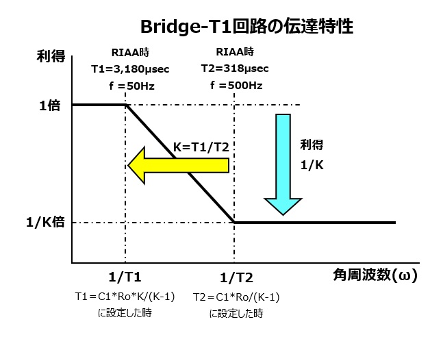
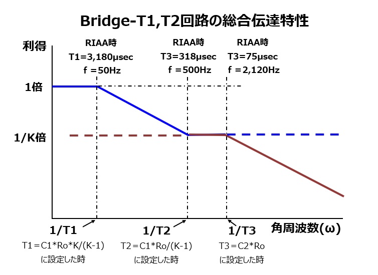
We were able to derive this. The transfer function A of this Bridge-T1 circuit has the characteristics of 1 pole (denominator) and 1 zero (numerator). This transfer function reproduces the low-frequency limit and turnover of the equalizer. We will consider roll-off again in the Bridge-T2 circuit. A=(1+jω＊C1Ro/(K-1)) / (1+jω(C1RoK/(K-1)) The denominator of the transfer function derives the low-frequency limit of 50Hz, and the numerator derives the turnover of 500Hz. In other words, the transfer function is matched to the equalizer characteristics by relating T1 to the ω in the denominator and T2 to the ω in the numerator. In the transfer function A in the above equation,

T1＝KC1Ro/(K-1) 　　　　　 Equation (2.27)
T2＝C1Ro/(K-1) 　　　　　 Equation (2.28)
T1/T2＝KC1Ro/(K-1)　/　C1Ro/(K-1)＝K

If you set it to be as in equation (2.29), what will the transfer function A be? When ω is 1/T1 A＝(jωC1Ro1/(K-1)+1) / (jωC1RoK/(K-1)+1) A(@T1)＝(j(1/T1)* C1Ro1/(K-1)+1) / (j(1/T1)C1RoK/(K-1)+1)
A(@T1)＝(j(1/(KC1Ro/(K-1))) C1Ro(1/(K-1)+1) / (j(1/(KC1Ro/(K-1)))C1RoK/(K-1)+1)
A(@T1)＝(j/K+1) / (j+1) Equation (2.30)
|A(@T1)|=SQRT((1/K^2+1^2)/(1^2+1^2)) Equation (2.31)
When ω is 1/T2
A(@T2)＝(j(1/T2) C1Ro1/(K-1)+1) / (j(1/T2)C1RoK/(K-1)+1)
A(@T2)＝(j(1/(C1Ro/(K-1)))* C1Ro1/(K-1)+1) / (j(1/( C1Ro/(K-1)))C1RoK/(K-1)+1)
A(@T1)=(j+1)/(jK+1) Equation (2.32)
|A(@T2)|＝SQRT((1^2+1^2)/(K^2+1^2)) Equation (2.33)

The gain of transfer function A starts to decrease at T1 = KC1Ro/(K-1) and drops to 1/K at T2 = C1Ro/(K-1). and then it becomes flat.

(That is, when the frequency is multiplied by K, the gain becomes 1/K.)

*In the case of RIAA, T1/T2=3180μsec/318μsec=10,
so K=10

|A(@T1)|＝SQRT((1/100+1)/2)≒1/SQRT(2)　
Start of the descent (3dB drop)

|A(@T2)|＝SQRT(２/100+1)　≒SQRT(2)/10　＝SQRT(2)/K　
End of the descent (3dB higher point before it reaches 1/K)

From the conditions derived so far, we will derive the LCR values ​​that make up the Bridge-T1 circuit of the RIAA equalizer.
Given
Ro = 600 Ω
For RIAA LCR equalizer
Low LIMIT 3180 μsec T1
Turn Over 318 μsec T2
Roll Off 75 μsec T3 (not used here)
From given
K = T1/T2 = 10
From conditions
L1/C1 = Ro^2
L1 = C1 * Ro^2
C1 = L1/Ro^2
R1 * (R1 + 2R3) = Ro^2
R1 = Ro (K-1)/(K+1)
R3＝Ro2K/(K^2-1)
T1=KC1R1/(K-1)
R1=600(10-1)/(10+1)＝490.91　（Ω）
R3=600210/(10^2-1)＝121.21　（Ω）

C1=T1(K-1)/(KRo)=3180/100000.9/600
＝0.0000477　　（F）
L1=R0^2*C1＝1.72　　（H）
Now we can calculate the constants of the LCR that make up Bridge-T1.

Analysis of Bridge-T2 circuit
Next, we will consider the Bridge-T2 circuit.
The Bridge-T2 circuit is a constant impedance low-pass filter like Bridge-T1, but this circuit only needs to achieve high-frequency roll-off, which means it has only one pole and no zero is required. As a result, it differs from the Bridge-T1 circuit in that it does not contain a resistor equivalent to R3. To simplify the analysis, we will provisionally set a resistor Rx equivalent to R3 in the Bridge-T1 circuit, and then finally set Rx to 0 to determine the LCR constants.
First, we substitute the results of Bridge-T1:

L2/C2＝Ro^2 　　　　　Equation (3.1)
L2=C2Ro^2 　　　　　Equation (3.2)
C2=L2/Ro^2 　　　　　Equation (3.3)
R2(Rx+2Rx)＝Ro^2＝Z1(Z1+2Zm) 　　　　　 Equation (3.4)
R2=Ro(K-1)/(K+1) 　　　　　 Equation (3.5)
Rx＝Ro2K/(K^2-1) 　　　　　 Equation (3.6)

As for the transfer function A,

A=(1+jω＊C2Ro/(K-1)) / (1+jω(C2RoK/(K-1)) Equation (3.7)
For the damping rate K of Bridge-T2, if we set the fictitious T4, which is not necessary for roll-off, to 1/100 of T3=75μsec (2120Hz), then K will be 100. Even with K=100, we can still say that 1/K≒0, K/(K-1)≒1, and it is possible to make T4 smaller and closer to 0, so this is considered to be equivalent to setting K=∞.
If we set the damping rate K=∞ here, then from Equation (3.5),

R2=Ro(K-1)/(K+1) K⇒∞,
(K-1)/(K+1)＝1 Therefore,

R2=Ro Equation (3.8)

From Equation (3.6),

R4＝Ro2K/(K^2-1) K⇒∞,
2K/(K^2-1)＝0
Therefore,
Rx＝0 Equation (3.9)
Also, since we can approximate 1/(K-1)＝0,
K/(K-1)＝1,
we can derive

A=(1+j0) / (1+jω(C2Ro))
A-1 / (1+jωc2*Ro) 　　 Equation (3.10)
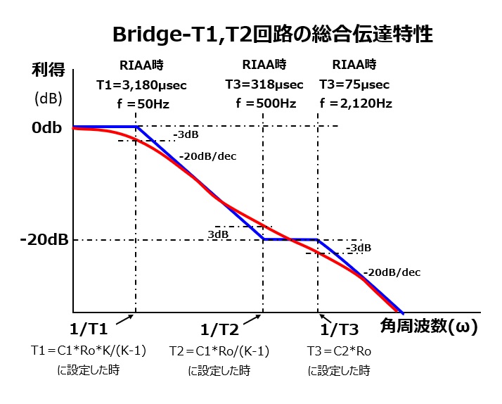
This transfer function has only one pole and no zero point.
In other words, this transfer function attenuates at a rate of 20dB/dec in the band above the cutoff frequency specified by T3.

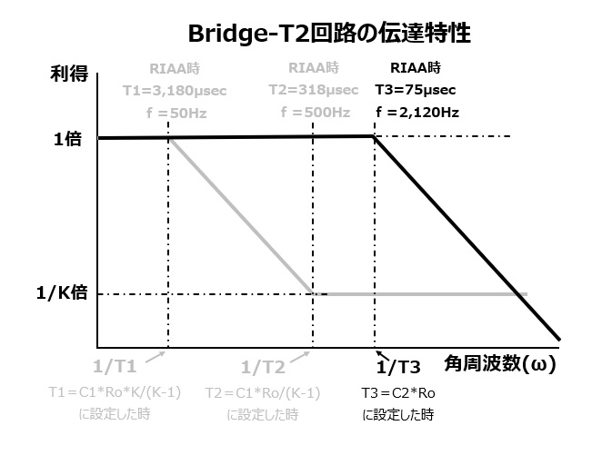
*The 1/K times notation on the Y axis of the graph above is for Bridge-T1 and is unrelated to Bridge-T2.
We will also calculate the various LCR settings of the RIAA equalizer for the Bridge-T2 circuit.

T3=C2Ro 75(μsec)＝C2600
C2=75/600　(μF)＝0.125　(μF)
L2=Ro^2C2 thus L2=360,0000.125*10^(-6)
＝0.045　(H)

Analysis of the entire circuit
When the Bridge-T1 and T2 circuits are viewed as a whole, the overall transfer function A(total) is
A(total)=A(Bridge-T1)A(Bridge-T2) so from equations (2.26) and (3.10), A(total)= A＝(jωC1Ro1/(K-1)+1) / ((jωC1Ro*K/(K-1)+1) * (1+j0) / (1+jω(C2Ro))
A(total)= A＝(jωC1Ro1/(K-1)+1) / ((jωC1RoK/(K-1)+1) * (1+jωC2*Ro) )　　Equation (4.1)
The transfer function now has a form with 2 poles and 1 zero.

Application to other equalizer curves
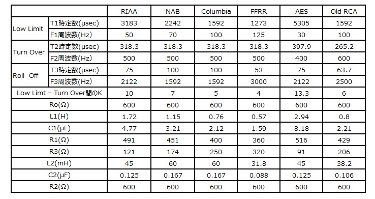
To support playback curves other than RIAA, calculate the LCR constants under the same conditions as the T1, T2, and T3 values ​​specified for each curve.
The calculation results for each LCR constant corresponding to RIAA and other standards in the original circuit format are shown below.

The LCR values ​​corresponding to each equalizer curve calculated here are merely calculation results and do not guarantee the characteristics.

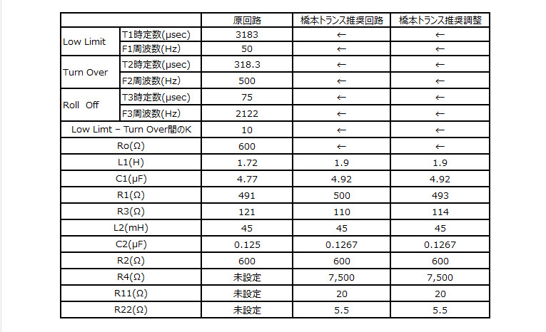
About the LCR constant setting in the recommended circuit of Hashimoto Transformer’s RIAA equalizer coil
So far, we have considered the original filter circuit consisting of two stages of constant impedance bridges. There are differences between Hashimoto Transformer’s recommended circuit and the original circuit, and the coil actually used has a DC resistance, which is also listed.
(The internal resistance of the coil is ignored in the calculation of the original circuit)

Figure: Hashimoto Transformer’s recommended circuit
In addition, the inductance value of the coil is different from the constant of the original circuit, and slightly different values ​​are recommended for other C and R.

What kind of curve can actually be reproduced if these values ​​are different from the original circuit?
The recommended circuit has a resistor R4 = 7.5kΩ in parallel with C1. How does the operation of the original circuit change when this resistor is inserted?
In the original circuit, as the frequency decreases, 1/(jωC1) gradually increases and becomes infinite at frequency 0.
In the area where 1/(jωC1) = ∞, the current flowing into the R3 side of the T circuit becomes zero. However, since a 7.5kΩ resistor is connected in parallel to C1, the earth shunt side is not open, and a voltage drop occurs due to the resistance, mitigating the effect of C1.
This acts in the direction of decreasing the output in the low frequency range compared to the curve of the original circuit.
Let’s simulate the transfer function of the recommended circuit of the Hashimoto transformer in Excel and check the output deviation.
When calculating the original circuit, we will substitute 500MΩ for R4 to make it almost negligible.
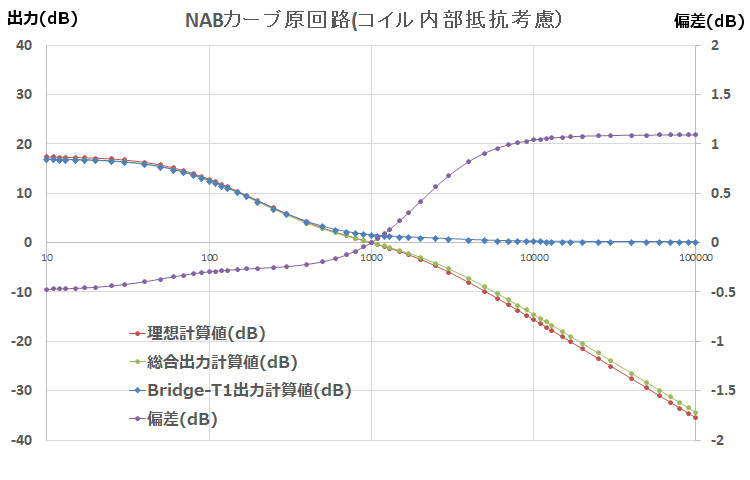
First, to confirm that this simulator is calculating correctly, we performed a calculation in the ideal state where the coil resistance is 0 in the original circuit.

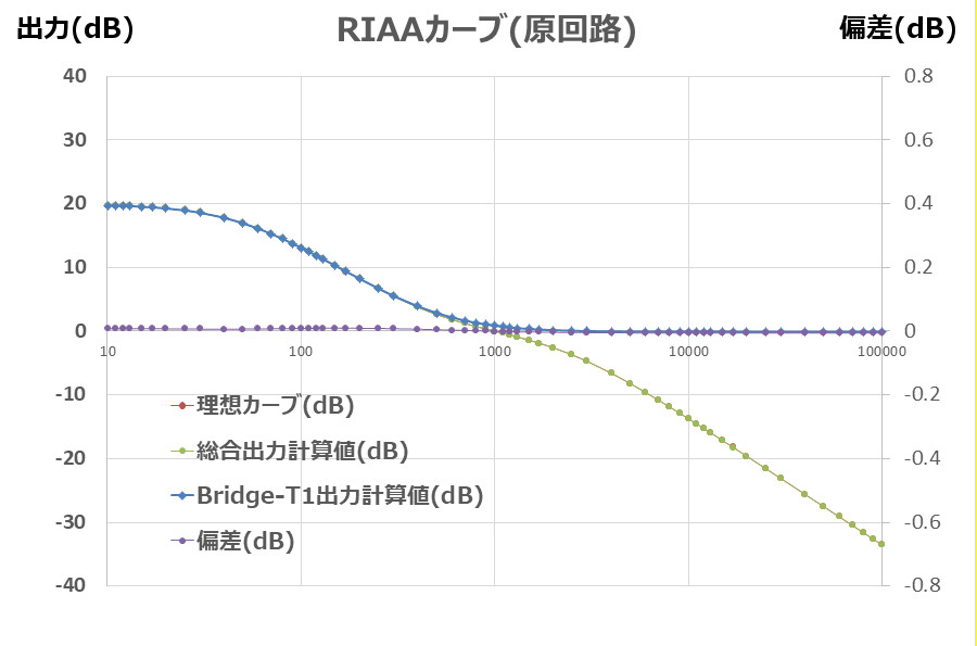
Since the coil has no resistance, there is almost no error (deviation) between the RIAA ideal calculation value and the result of the circuit simulator.
Next, we will calculate the original circuit by taking into account the coil resistance.

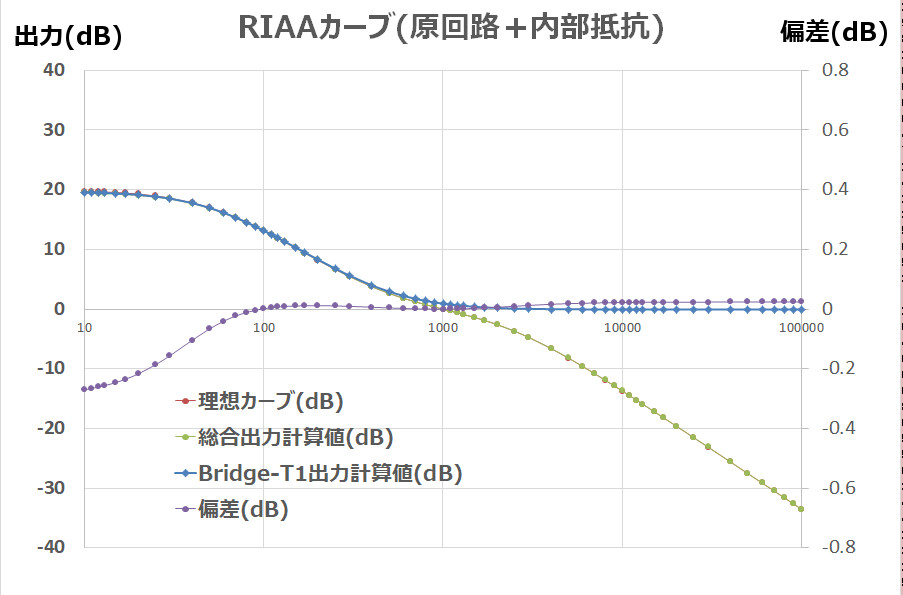
By taking the internal resistance into account, a tendency for a decrease was observed in the low range below 100Hz, and a deviation of about -0.27dB was observed at 10Hz. (The L value is the theoretically calculated value of 1.72H, and the resistance used in the calculation is 18.1Ω.)

Next, we will show the results of a simulation using the LCR values ​​recommended by Hashimoto Transformers.

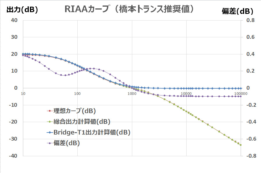
The deviation fluctuates on the positive side in the zone below 1kHz, and the maximum deviation in the low range is +0.4dB at 10Hz.
The result of simply taking the internal resistance into account in the calculation value of the original circuit has a simpler curve and less deviation than the value recommended by Hashimoto Transformers. I’m sure there is a reason for this…

I’m a little concerned about the positive undulation in the low range and the drop in the high range (although it’s only 0.1dB).
The theoretical values ​​of L1 and L2 to obtain RIAA characteristics are 1.72H and 45mH, while the L values ​​of the Hashimoto transformer are 1.9H and 45mH, respectively, with only L1 being a larger value. The Hashimoto transformer may have wanted to control the characteristics in the direction of raising the low frequencies, or it may have used settings that were easy to combine, considering that the combined resistors and capacitor capacities are restricted by the E24 series, etc.
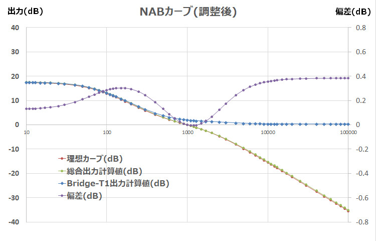
This time, using the coil value and internal resistance value of the Hashimoto transformer, I tried cutting and trying to find the C and R settings that would minimize the deviation.
As a result, I was able to obtain fairly straightforward characteristics with the condition settings on the right of the table below.

Because I tried cutting and trying, I’m sure there are better combinations of settings.
The characteristics obtained are as follows.

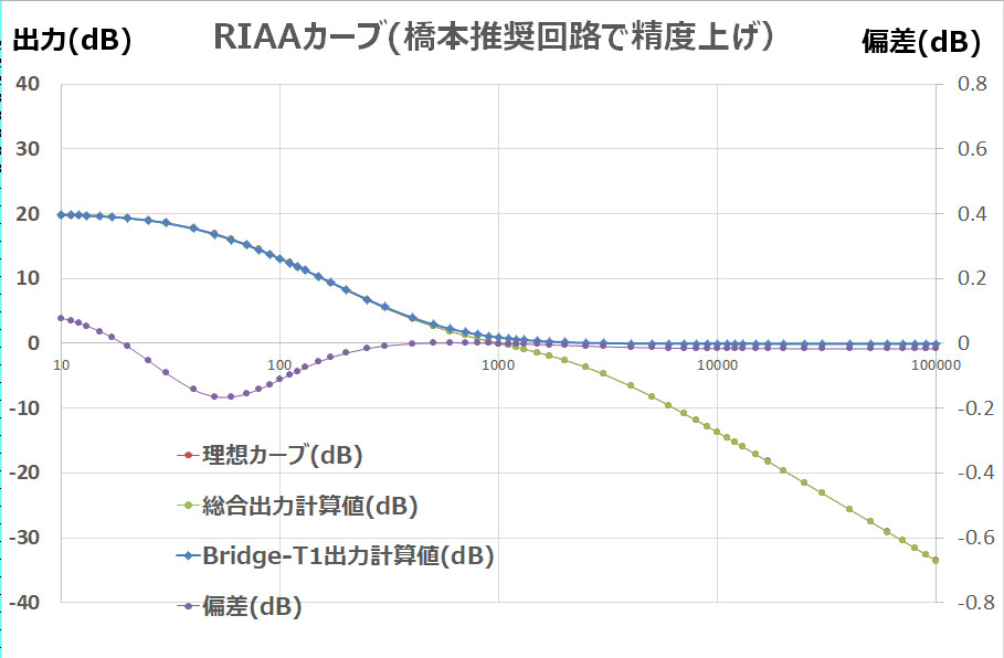
There is a drop of less than -0.2dB around 50-60Hz, but the -0.1dB drop seen in the high frequencies above 1kHz has been eliminated.

Support for other equalizing curves
This time, we are focusing on RIAA and considering other equalizing curves.

The output characteristics of the various curves are shown here.

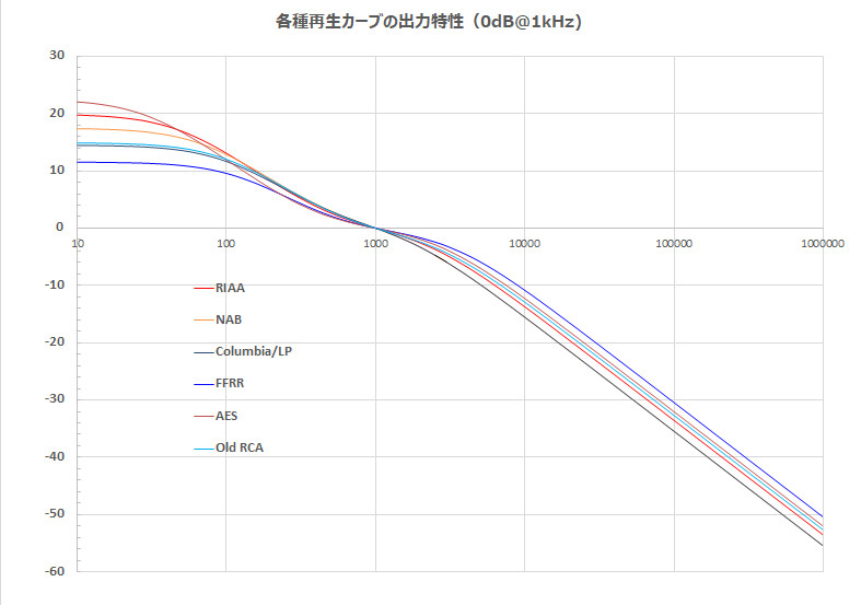
①NAB
I substituted the theoretical LCR value into the original circuit and calculated it taking into account the internal resistance.
R1= 451 Ω
R2= 600 Ω
R3= 174 Ω
R4= 500MΩ
Ro= 600 Ω
R11=12.1 Ω
R22=4.4 Ω
L1= 1.15 H
L2= 0.06 H
C1= 3.21 μF
C2= 0.125 μF

If the deviation at 1kHz is 0dB, the high range shows an output increase of more than 1dB on the + side, while the low range shows an opposite trend of -0.5dB at 10Hz, with an overall tendency to increase in the high range.
The deviation is large as it is, so I adjusted the LCR value by cut and try.
R1= 450 Ω
R2= 600 Ω
R3= 160 Ω
R4= 25000 Ω
Ro= 600 Ω
R11=12.1 Ω
R22=4.4 Ω
L1= 1.15 H
L2= 0.069 H
C1= 3.3063 μF
C2= 0.134 μF

When the deviation at 1 kHz is set to 0 dB, the high frequency side is +0.4 dB, and the low frequency side is +0.3 dB, although there is some undulation. The deviation at 1 kHz is set to 0, but when the center is moved to the +0.2 dB side, the deviation is within ±0.2 dB in the entire band. Since this is not actually being manufactured and the provisionally set internal resistance value is not accurate, this is the end of the NAB adjustment.

②COLUMBIA / LP
R1= 400 Ω
R2= 600 Ω
R3= 250 Ω
R4= 500MΩ
Ro= 600 Ω
R11=8 Ω
R22=5 Ω
L1= 0.76 H
L2= 0.06 H
C1= 2.12 μF
C2= 0.1668 μF

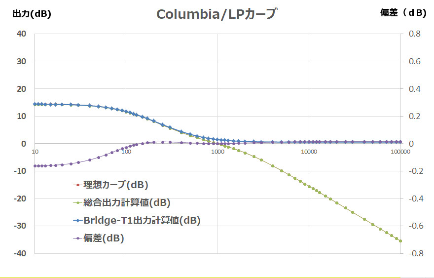
The Columbia/LP curve is a combination of theoretical values ​​and internal resistance, with almost zero deviation on the high-frequency side and -0.2 dB (@10 Hz) on the low-frequency side, so no further adjustment is required.

③FFRR curve
R1= 360 Ω
R2= 600 Ω
R3= 320 Ω
R4= 500MΩ
Ro= 600 Ω
R11=6 Ω
R22=5 Ω
L1= 0.57 H
L2= 0.032 H
C1= 1.59 μF
C2= 0.088 μF

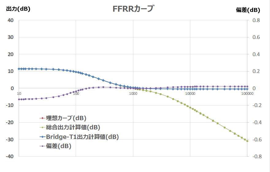
FFRR also has an output characteristic deviation well within 0.2 dB, so this is also OK.

④AES curve
R1= 516 Ω
R2= 600 Ω
R3= 91 Ω
R4= 500MΩ
Ro= 600 Ω
R11=30 Ω
R22=5.5 Ω
L1= 2.94 H
L2= 0.045 H
C1= 8.18 μF
C2= 0.125 μF

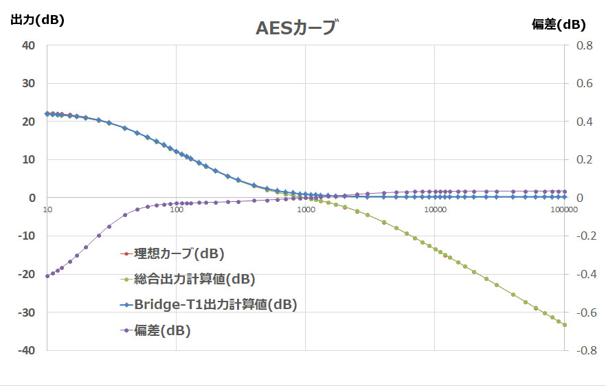
The deviation spreads to -0.4dB at 10Hz, but is within -0.2dB up to 25Hz.

⑤OLD RCA curve
R1= 429 Ω
R2= 600 Ω
R3= 206 Ω
R4= 500MΩ
Ro= 600 Ω
R11=12 Ω
R22=5.5 Ω
L1= 0.8 H
L2= 0.038 H
C1= 2.21 μF
C2= 0.106 μF

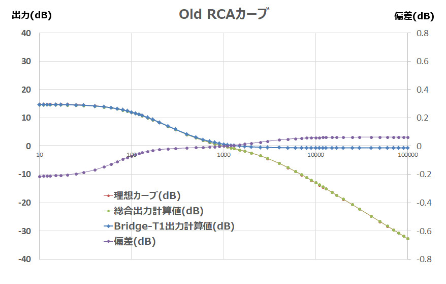
There is a slight tendency for the highs to rise overall, but the deviation is within 0.2dB on the negative side and 0.1dB on the positive side, so this is also the end.

The discussion on LCR phono equalizers ends here for now.

*The LCR setting values ​​for each curve derived this time are merely calculated values ​​and do not guarantee the actual characteristics, so please refer to them at your own risk. Also, if you find any errors in the thinking or calculation results, please contact us.